Replace b with \( \bar{y} - m\bar{x} \)
\( \sum_{i=1}^n x_i y_i - b \sum_{i=1}^n x_i = \sum_{i=1}^n x_i y_i - (\bar{y} - m\bar{x}) \sum_{i=1}^n x_i \)
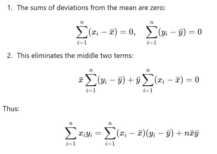
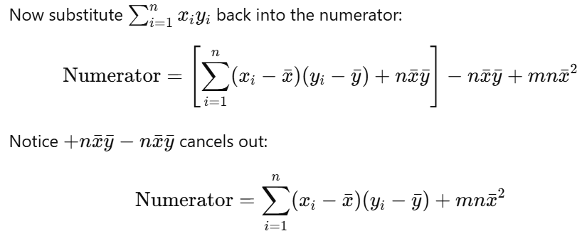
Substituting into numerator
\( \sum_{i=1}^n x_i y_i - b \sum_{i=1}^n x_i = \sum_{i=1}^n x_i y_i - (\bar{y} - m\bar{x}) \sum_{i=1}^n x_i \)
Expand the numerator
\( \sum_{i=1}^n x_i y_i - (\bar{y} - m\bar{x}) \sum_{i=1}^n x_i = \sum_{i=1}^n x_i y_i - \bar{y} \sum_{i=1}^n x_i + m\bar{x} \sum_{i=1}^n x_i \)
simplified numerator
\( \sum_{i=1}^n x_i y_i - \bar{y} \sum_{i=1}^n x_i + m \bar{x} \sum_{i=1}^n x_i
\)
\( \sum_{i=1}^n x_i y_i - n\bar{y}\bar{x} + m \bar{x}^2 \)
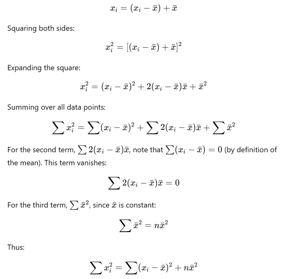
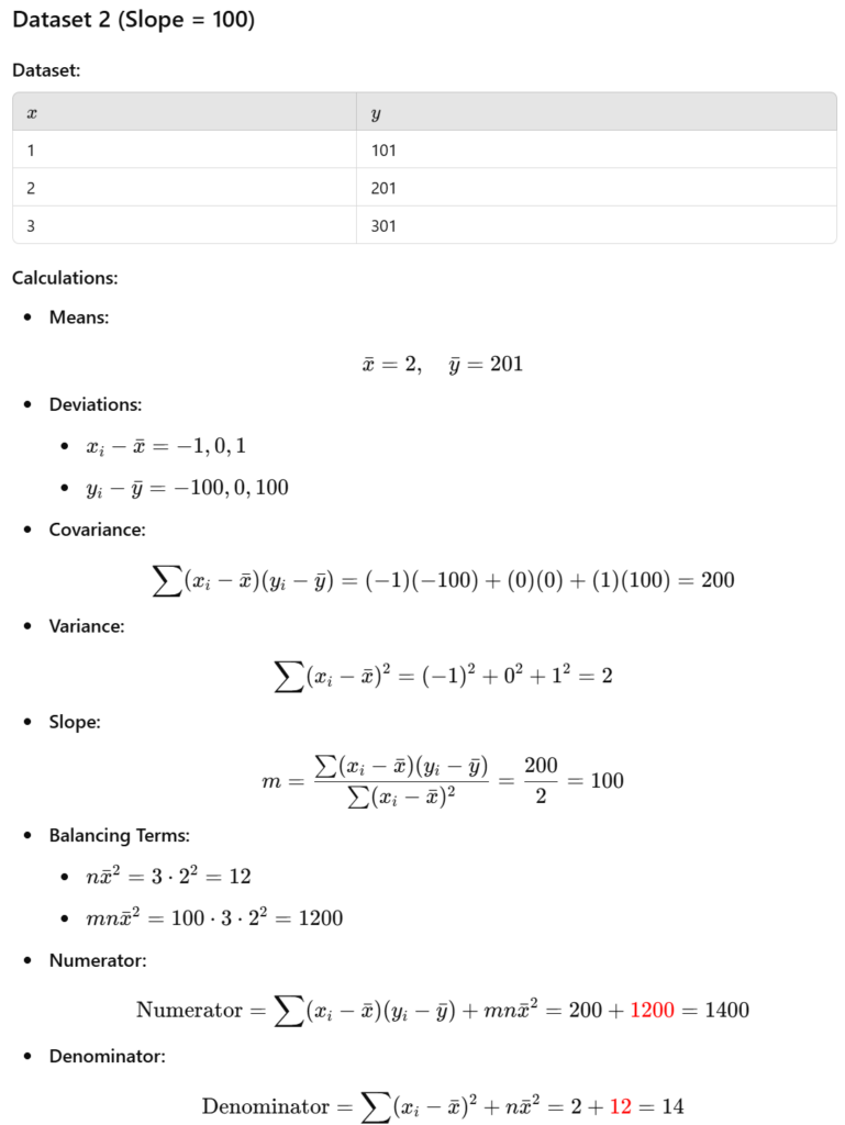
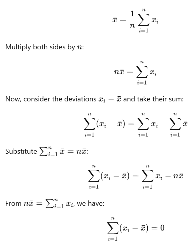
See fundamenals below for \( \sum_{i=1}^n x_i = n \bar{x} \)
well articulated